Flow Matching Policy Gradients
Simple Online Reinforcement Learning with Flow Matching
Chung Min Kim Ethan Weber Haven Feng Angjoo Kanazawa
Flow models have become the go-to approach to model distributions in continuous space. They soak up data with a simple, scalable denoising objective and now represent the state-of-the art in generating images, videos, audio and, more recently, robot action. However, they are still unpopular for learning from rewards through reinforcement learning.
Meanwhile, to perform RL in continuous spaces, practicioners typically train far simpler Gaussian policies, which represent a single, ellipsoidal mode of the action distribution. Flow-based policies can capture complex, multimodal action distributions, but they are primarily trained in a supervised manner with behavior cloning (BC). We show that it’s possible to train RL policies using flow matching, the framework behind modern diffusion and flow models, to benefit from its expressivity.
We approached this project as researchers primarily familiar with diffusion models. While working on VideoMimic, we felt limited by the expressiveness of Gaussian policies and thought diffusion could help. In this blog post, we’ll explain how we connect flow matching and on-policy RL in a way that makes sense without an extensive RL background.
We introduce Flow Policy Optimization (FPO), a new algorithm to train RL policies with flow matching. It can train expressive flow policies from only rewards. We find its particularly useful to learn underconditioned policies, like humanoid locomotion with simple joystick commands.
Flow Matching
Flow matching optimizes a model to transform a simple distribution (e.g., the Gaussian distribution) into a complex one through a multi-step mapping called the marginal flow. We expand on the marginal flow in more detail in another blog post for Decentralized Diffusion Models. The flow smoothly directs a particle $x_t$ to the data distribution, so integrating the flow across time leads to a data sample. We can actually calculate the marginal flow analytically, which we do in real-time in the plot below:
Each particle here represent an $x_t$ noisy latent that gets iteratively denoised as the time goes from zero to one. If you’re on desktop, drag the control points of the modes on the right to see how the underlying PDF and the particle trajectories change. Notice how the probability mass flows smoothly from the initial noise to form two distinct modes. The multi-step mapping is the magic that lets flow models transform a simple, tractable distribution into one of arbitrary complexity.
While it’s simple to compute this flow in 1D, it becomes intractable over large datasets in high dimensional space. Instead, we use flow matching, which compresses the marginal flow into a neural network through a simple reconstruction objective.

Flow matching perturbs a clean data sample with Gaussian noise then tasks the model with reconstructing the sample by predicting the velocity, which is the derivative of $x_t$’s position w.r.t. time. In expectation over a fixed dataset, this optimization recovers the marginal flow for any $x_t$. Integrating $x_t$’s position across time along the marginal flow will recover a sample from the data distribution.
Geometrically, the marginal flow points to a weighted-average of the data where the weights are a function of the timestep and distance from $x_t$ to each data point. You can see the particles follow the marginal flow exactly in the plot above when stochasticity is turned off. Stated simply, flow matching learns to point the model’s flow field, $v_t(x_t)$, to the data distribution.
Flow matching has statistical signifigance too. Instead of computing exact likelihoods (expensive and unstable), it optimizes a lower bound called the Evidence Lower Bound (ELBO). This pushes the model toward higher likelihoods without computing them directly. In the limit, the flow model will sample exactly from the probability distribution of the dataset. So if you’ve learned the flow function well, you’ve learned the underlying structure of the data.
Flowing toward a data point increases its likelihood under the model.
On-Policy RL: Sample, Score, Reinforce
On-policy reinforcement learning follows a basic core loop: sample from your policy, score each action with rewards, then make high-reward actions more likely. Rinse and repeat.
This procedure climbs the policy gradient—the gradient of expected cumulative reward. Your model collects “experience” from by sampling its learned distribution, sees which samples are most advantageous, and adjusts to perform similar actions more often.
On-policy RL can be cast as search iteratively distilled into a model. The policy “happens upon” good behaviors through exploration, then reinforces them. Over time, it discovers the patterns in the random successes and develops reliable strategies. You can start from a pretrained model and continue training with RL to explore within a rich prior rather than at random. This is the dominant approach to upcycle LLMs for preference alignment and reasoning.
Image Generation Analogy
Here’s an example RL loop to understand (replace with DMControl rollout videos from Brent):
- Generate a batch of images from your model (rollouts)
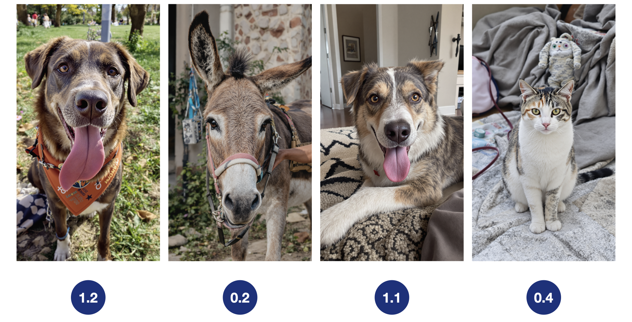
- Score each image with a reward (maybe “how much does this look like a dog?”)
- Train your model to boost the likelihood of high-scoring images
- Repeat until your model reliably generates high-reward images
Sample and score images:
From the rewards, we calculate advantages. These can be viewed as the reward normalized w.r.t. the expected reward from the rest of the rollout under the current policy. This expected reward is what you learn with a critic in PPO
Calculate each advantage and form policy gradient:
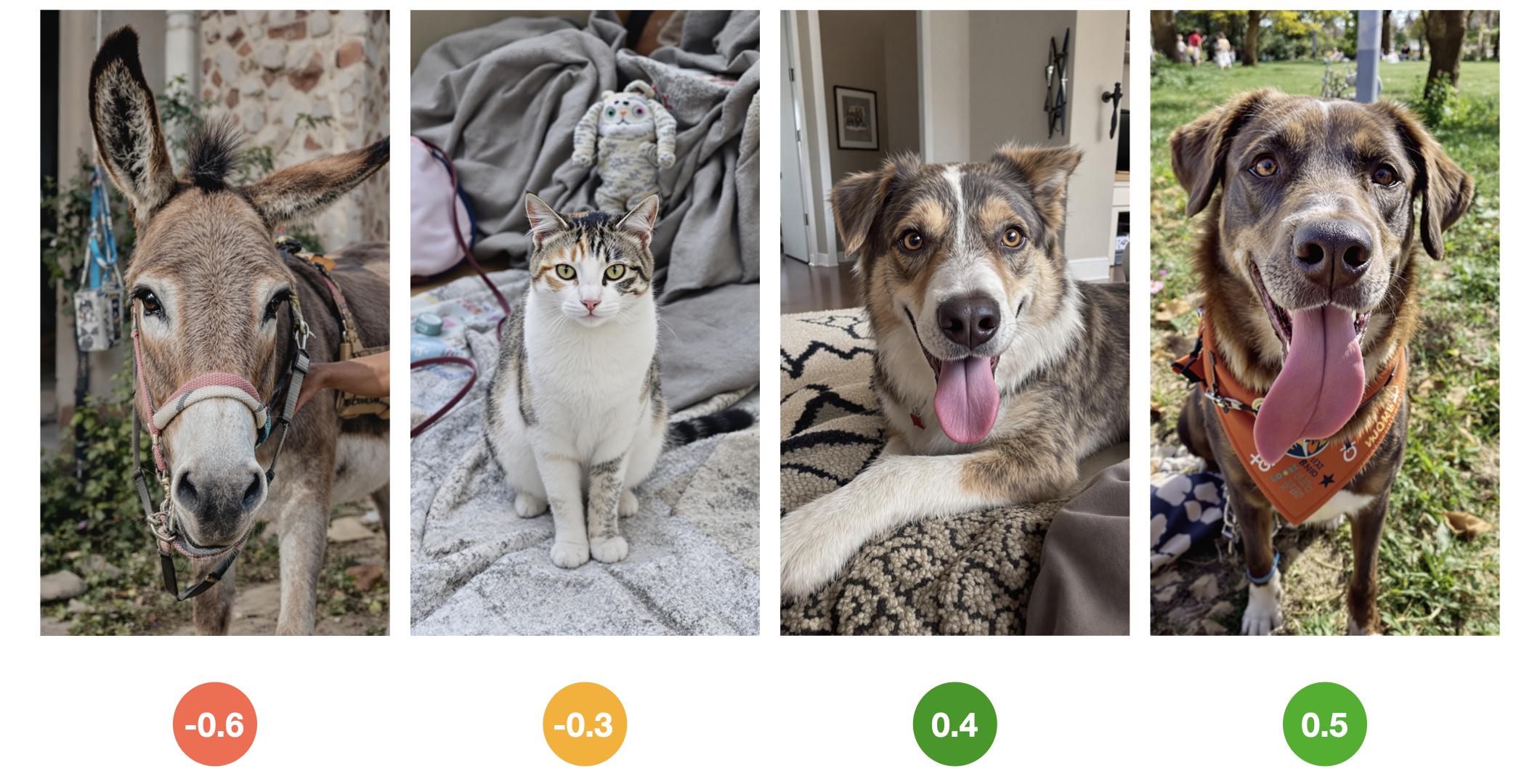
Given the advantages, train the model on each data point with a gradient update scaled by the corresponding advantage. So, if the advantage is negative, it will become less likely. Postive advantage, more likely.
Flow Matching Policy Gradients
To reiterate, the goal of on-policy RL is simple: increase the likelihood of high-reward actions. Meanwhile, flow matching naturally increases likelihoods by redirecting probability flow toward training samples. This makes our objective clear—redirect the flow toward high reward actions.
In the limit of perfect optimization, flow matching assigns probabilities according to the frequency of samples in your training set. Since we’re using RL, that “training set” is dynamically generated from the model.
Advantages make the connection between synthetic data generation and on-policy RL explicit. In RL, we calculate the advantage of each sampled action, a quantity that indicates how much better it was than expected. These advantages are centered around zero to reduce variance: positive for better-than-expected actions, negative for worse. Advantages then become a loss weighting in the policy gradient. As a simple example, if an action is very advantageous, the model encounters a scaled-up loss on it and learns to boost it aggressively.

Zero-mean advantages are fine for RL in discrete spaces because a negative advantage simply pushes down the logit of a suboptimal action, and the softmax ensures that the resulting action probabilities remain valid and non-negative. Flow matching, however, learns probability flows to sample from a training data distribution. These must be nonnegative by construction, so negative loss weights break the interpretation.
There’s a simple solution: make the advantages nonnegative. Shifting advantages by a constant doesn’t change the policy gradient. In fact, this is the mathematical property that lets us use advantages instead of raw rewards in the first place. Here’s how we can understand non-negative advantages in the flow matching framework:

Advantages manifest as loss-weighting, which can be intuitively expressed in the marginal flow framework. The marginal flow is the weighted average of the paths (the $u_t$’s) from the current noisy particle, $x_t$, to each data point $x$. The paths are also weighed by $q(x)$, the probability of drawing $x$ from your training set. This is typically a constant $\frac{1}{N}$ for a dataset of size $N$, assuming every data point is unique. Loss weights are equivalent to altering the frequency of the data points in your training set. If the loss for a data point is scaled by a factor of 2, its equivalent to that data point showing up twice in the train set.
Now, we can get a complete picture of the algorithm that connects flow matching and reinforcement learning:
- Generate actions from your flow model using your choice of sampler
- Score them with rewards and compute advantages
- Flow match on the advantage-weighed actions
This procedure boosts the likelihood of actions that achieve high reward while preserving the desirable properties of flow models—multimodality, expressivity and the improved exploration that stems from them. We visualize the procedure below in the same 1D flow diagram as above:
Acknowledgements
We thank Qiyang (Colin) Li, Oleg Rybkin, Lily Goli and Michael Psenka for helpful discussions and feedback on the manuscript. We thank Arthur Allshire, Tero Karras, Miika Aittala, Kevin Zakka and Seohong Park for insightful input and feedback on implementation details and the broader context of this work.